Forecasting
Study these flashcardsFree · spaced repetition · iPhone, Android, Mac & web
All cards
1
What are the 3 main forecasting techniques
The high low method
Linear regression
Time series analysis
Linear regression
Time series analysis
2
Explain the high low method
The high low method involves using the hughest and lowest values to calculate the fixed and variable elements of cost/income.
3
Explain linear regression in forecasting
uses a formula to
estimate the linear relationship between the two variables as follows:
y = a +bx
where
y = dependant variable
a = interception (on y-axis)
b = gradient
x = independant variable
The regression equation can be used for predicting values of y from a given x value
The reliability of these forecasts will depend on the strength of the relationship between the two variables. The strength is known as correlation.
estimate the linear relationship between the two variables as follows:
y = a +bx
where
y = dependant variable
a = interception (on y-axis)
b = gradient
x = independant variable
The regression equation can be used for predicting values of y from a given x value
The reliability of these forecasts will depend on the strength of the relationship between the two variables. The strength is known as correlation.
4
Explain correlation
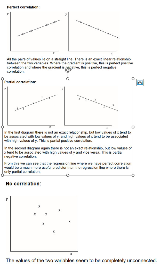
Two variables are said to be correlated if they are related to one another, or,
more precisely, if changes in the value of one tend to accompany changes in
the other.
Degrees of correlation
Two variables might be:
• perfectly correlated
• partially correlated
• uncorrelated.
more precisely, if changes in the value of one tend to accompany changes in
the other.
Degrees of correlation
Two variables might be:
• perfectly correlated
• partially correlated
• uncorrelated.
5
Explain correlation coefficient
Care must be taken when making predictions based on historical data.
Regression analysis assumes perfect linear relationships; but where this is not
the case, the predictions may not be able to be relied upon.
It is therefore important to measure the strength of the correlation, which can
be done by calculating the Pearsonian correlation coefficient, r.
r must always be between -1 and +1.
If r = +1, there is perfect positive linear correlation
If r = 0, there is no linear correlation
If r = -1, there is perfect negative linear correlation
For other values of r, the meaning is not so clear. It is generally taken that if r >
+0.8, then there is strong positive correlation and if r < -0.8, there is strong
negative correlation, however more meaningful information can be gathered
from calculating the coefficient of determination, r2
Regression analysis assumes perfect linear relationships; but where this is not
the case, the predictions may not be able to be relied upon.
It is therefore important to measure the strength of the correlation, which can
be done by calculating the Pearsonian correlation coefficient, r.
r must always be between -1 and +1.
If r = +1, there is perfect positive linear correlation
If r = 0, there is no linear correlation
If r = -1, there is perfect negative linear correlation
For other values of r, the meaning is not so clear. It is generally taken that if r >
+0.8, then there is strong positive correlation and if r < -0.8, there is strong
negative correlation, however more meaningful information can be gathered
from calculating the coefficient of determination, r2
6
Explain coefficient of determination
This measures how good the estimated regression equation is, designated as
r 2 . The higher the r2 value, the more confidence one can have in the regression
equation. Statistically, the coefficient of determination represents the proportion
of the total variation in the y variable that is explained by the regression
equation. It has the range of values between 0 and 1.
If result is 0.9 that means 90% of the result can be explained by the regression equation but 10% was something unknown
r 2 . The higher the r2 value, the more confidence one can have in the regression
equation. Statistically, the coefficient of determination represents the proportion
of the total variation in the y variable that is explained by the regression
equation. It has the range of values between 0 and 1.
If result is 0.9 that means 90% of the result can be explained by the regression equation but 10% was something unknown
7
• Assumes a linear relationship between the variables.
• Only measures the relationship between two variables. In reality the
dependent variable is affected by many independent variables.
• Only interpolated forecasts tend to be reliable. The equation should not be
used for extrapolation.
• Regression assumes that the historical behaviour of the data continues
into the foreseeable future.
• Interpolated predictions are only reliable if there is a significant correlation
between the data.
• Ignores inflation
What are the limitations of linear regression
• Assumes a linear relationship between the variables.
• Only measures the relationship between two variables. In reality the
dependent variable is affected by many independent variables.
• Only interpolated forecasts tend to be reliable. The equation should not be
used for extrapolation.
• Regression assumes that the historical behaviour of the data continues
into the foreseeable future.
• Interpolated predictions are only reliable if there is a significant correlation
between the data.
• Ignores inflation
8
Explain interpolation and extrapolation
1 If the value of x is within the range of our original data, the
prediction is known as Interpolation.
2 If the value of x is outside the range of our original data, the
prediction is known as Extrapolation.
In general, interpolation is much safer than extrapolation.
prediction is known as Interpolation.
2 If the value of x is outside the range of our original data, the
prediction is known as Extrapolation.
In general, interpolation is much safer than extrapolation.
9
Explain Time series analysis
A time series is a series of values for a variable which changes over time.
Where the variable is subject to ‘seasonal’ variations, it will be measured at
regular intervals.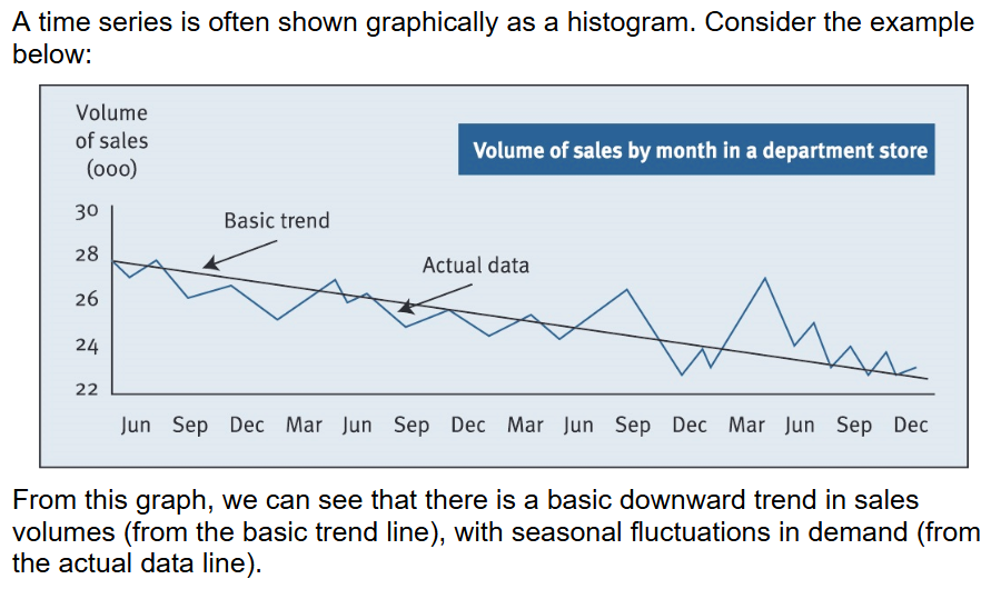
Where the variable is subject to ‘seasonal’ variations, it will be measured at
regular intervals.
10
Using linear regression in time series
Y = total sales
A = sales at the point you started recording
B = period
x = income/profit per sale
A = sales at the point you started recording
B = period
x = income/profit per sale
11
What are the components of time series analysis
A time series has four components:
1 The basic trend (T)
2 Seasonal variations (S)
3 Cyclical variations (C)
4 Residual variations (R)
1 The basic trend (T)
2 Seasonal variations (S)
3 Cyclical variations (C)
4 Residual variations (R)
12
Explain the basic trend in time series analysis
The basic trend (long-term)
The basic trend refers to the general direction of the graph of a time series over
a long interval of time, once the short-term variations have been smoothed out.
We will see how to determine the underlying basic trend later in this section
The basic trend refers to the general direction of the graph of a time series over
a long interval of time, once the short-term variations have been smoothed out.
We will see how to determine the underlying basic trend later in this section
13
Explain the seasonal variations in time series analysis
Seasonal variations (short-term)
Seasonal variations are short-term fluctuations in value due to different
circumstances which occur at different times of the year, on different days of the
week, different times of day, etc. Some examples might be:
• Ice cream sales are highest in summer
• Sales of groceries are highest on Saturdays
• Traffic is greatest in the morning and evening rush hours
Seasonal variations are short-term fluctuations in value due to different
circumstances which occur at different times of the year, on different days of the
week, different times of day, etc. Some examples might be:
• Ice cream sales are highest in summer
• Sales of groceries are highest on Saturdays
• Traffic is greatest in the morning and evening rush hours
14
Explain cyclical variations in time series analysis
Cyclical variations (medium-term to long-term)
Cyclical variations are medium-term to long term fluctuations about the basic
trend. These cycles are rarely of consistent length and do not necessarily follow
similar patterns. Cyclical variations are usually associated with the economy,
such as intervals of boom, decline, recession and recovery. We would need 6 or
7 full cycles of data to be sure that the cycle was there
Cyclical variations are medium-term to long term fluctuations about the basic
trend. These cycles are rarely of consistent length and do not necessarily follow
similar patterns. Cyclical variations are usually associated with the economy,
such as intervals of boom, decline, recession and recovery. We would need 6 or
7 full cycles of data to be sure that the cycle was there
15
Explain residual random variations in time series analysis
Residual or random variations (short-term)
Residual variations are the irregular items due to chance events such as
pandemics, floods, strikes etc. By their very nature, they are unpredictable and
therefore cannot play a large part in forecasting.
The residual is the difference between the actual value and the figure predicted
using the trend, the cyclical variation and the seasonal variation. It is important
to extract any significant residual variations from the time series data before
using them for forecasting
Residual variations are the irregular items due to chance events such as
pandemics, floods, strikes etc. By their very nature, they are unpredictable and
therefore cannot play a large part in forecasting.
The residual is the difference between the actual value and the figure predicted
using the trend, the cyclical variation and the seasonal variation. It is important
to extract any significant residual variations from the time series data before
using them for forecasting
16
How do you calculate the trend in time series analysis
There are three main methods of finding the underlying trend of the data:
1 Inspection. The trend line can be drawn by eye with the aim of plotting the
line so that it lies in the middle of the data.
2 Least squares regression analysis (and also high-low). The x axis
represents time and the periods of time are numbers, e.g. January is 1,
February is 2, March is 3, etc.
3 Moving averages. This method attempts to remove seasonal or cyclical
variations by a process of averaging.
1 Inspection. The trend line can be drawn by eye with the aim of plotting the
line so that it lies in the middle of the data.
2 Least squares regression analysis (and also high-low). The x axis
represents time and the periods of time are numbers, e.g. January is 1,
February is 2, March is 3, etc.
3 Moving averages. This method attempts to remove seasonal or cyclical
variations by a process of averaging.
17
Advantages and disadvantages of time series analysis
The advantages of forecasting using time series analysis are that:
• forecasts are based on clearly-understood assumptions
• trend lines can be reviewed after each successive time period,
when the most recent historical data is added to the analysis;
consequently, the reliability of the forecasts can be assessed
• forecasting accuracy can possibly be improved with experience.
The disadvantages of forecasting with time series analysis are that:
• there is an assumption that what has happened in the past is a
reliable guide to the future
• there is an assumption that a straight-line trend exists
• there is an assumption that seasonal variations are constant,
either in actual values using the additive model (such as dollars of
sales) or as a proportion of the trend line value using the
multiplicative model.
None of these assumptions might be valid.
However, the reliability of a forecasting method can be established over
time. If forecasts turn out to be inaccurate, management might decide
that they are not worth producing, and that different methods of
forecasting should be tried. On the other hand, if forecasts prove to be
reasonably accurate, management are likely to continue with the same
forecasting method.
• forecasts are based on clearly-understood assumptions
• trend lines can be reviewed after each successive time period,
when the most recent historical data is added to the analysis;
consequently, the reliability of the forecasts can be assessed
• forecasting accuracy can possibly be improved with experience.
The disadvantages of forecasting with time series analysis are that:
• there is an assumption that what has happened in the past is a
reliable guide to the future
• there is an assumption that a straight-line trend exists
• there is an assumption that seasonal variations are constant,
either in actual values using the additive model (such as dollars of
sales) or as a proportion of the trend line value using the
multiplicative model.
None of these assumptions might be valid.
However, the reliability of a forecasting method can be established over
time. If forecasts turn out to be inaccurate, management might decide
that they are not worth producing, and that different methods of
forecasting should be tried. On the other hand, if forecasts prove to be
reasonably accurate, management are likely to continue with the same
forecasting method.